| Dimension | EMH / Rational Expectations | Behavioral Finance |
|---|---|---|
| Core assumption about investors | Fully rational, unbiased, maximize expected utility | Bounded rationality, subject to systematic cognitive biases |
| How do prices form? | Prices immediately reflect all relevant information | Prices reflect biases + fundamentals; correction is slow and noisy |
| Are forecast errors random? | Yes — errors are random, mean zero, serially uncorrelated | No — errors can be systematic (overconfidence, anchoring, herding) |
| What happens to arbitrage? | Smart money eliminates any mispricing almost instantly | Arbitrage is *limited* — risk, noise traders, and capital constraints prevent full correction |
| Can systematic profits exist? | No — in the long run, you can't beat a random walk | Yes — momentum, value premium, and post-earnings drift persist |
| What drives excess volatility? | Doesn't exist — prices track fundamentals | Investor sentiment drives prices away from fundamentals |
| Policy implication | Don't interfere with markets; trust prices as signals | Investor protection and market design matter; nudges can improve outcomes |
| Nobel Laureates (related) | Eugene Fama (2013), Robert Lucas (1995) | Daniel Kahneman (2002), Richard Thaler (2017), Robert Shiller (2013) |
| Note: | ||
| Source: Mishkin 13e, Ch. 7, pp. 159–176. Behavioral finance does not claim markets are always wrong — it claims systematic biases prevent the kind of perfect efficiency the EMH describes. |
Behavioral Finance & Market Anomalies
ECON304-M01 — Money & Banking | Episode 3: The Architecture of Compliance
2026-03-23
“The Map Is Not the Territory.”
What if the market isn’t wrong?
What if you are?
That’s the brutal insight at the heart of behavioral finance, and it is, frankly, a more disturbing idea than market failure. Market failures can be fixed — you add regulators, you update the rules, you fire the fraudsters. But human cognition? That’s not a bug. It’s the operating system. And in the world of the Global Omni PanOpticon Corp, Logan Prime figured that out a long time ago.
He doesn’t need to force anyone to comply. He just has to understand how people’s brains actually work — and build the system around it.
“The PanOpticon doesn’t need walls. It needs anchors.”
— Patsy Leviathon, encrypted message fragment recovered from Node 7, Sector 12
Today, we build the economic framework that explains exactly what she meant.
Class Information
Part 1: Quick Review — Class #14 and the Bridge to Today
What We Built in Class #14
Last class, we completed the rationalist’s toolkit for stock valuation and market efficiency:
Note
The Class #14 Recap — Three Big Results
- One-Period Valuation Model: \(P_0 = \frac{Div_1 + P_1}{1 + k_e}\) — a stock’s fair value is the present value of next period’s dividend plus the expected resale price.
- Gordon Growth Model: \(P_0 = \frac{Div_1}{k_e - g}\) — extend the one-period model to perpetuity with constant dividend growth. Simple, powerful, and used everywhere.
- Efficient Market Hypothesis (EMH): Three forms:
- Weak: Current prices fully reflect all past trading information (no technical analysis profits)
- Semi-strong: Current prices fully reflect all publicly available information (no fundamental analysis profits)
- Strong: Current prices fully reflect all information, including private/insider information
Source: Frederic S. Mishkin,3 Ch. 7, pp. 147–157.
The rational expectations framework underlying the EMH makes a breathtaking claim: markets get prices right, on average, because smart investors will arbitrage away any systematic errors.
Today we ask: what happens when the smart investors are also human?
Today’s Central Question
The EMH assumes investors behave like the economics textbook’s favorite fictional creature: Homo economicus — perfectly rational, fully informed, immune to emotion, processing probability distributions like a quantum computer.
Behavioral finance asks: what if they don’t? What if they can’t?
And more darkly: what if someone knows they don’t — and builds a control system around it?
Tip
PanOpticon System Alert — Episode 3 Begins
[PanOpticon encrypted transmission, Node 7-Alpha, timestamp 0317:44]
Patsy — I need you to see what I’ve found. Logan Prime’s ROI document from Class 10 isn’t just about calculating who deserves resources. That’s the output. The input is more sophisticated. He’s not measuring actual welfare. He’s measuring compliance scores — and he’s designed the entire scoring system to exploit exactly how human brains mis-process information.
The population isn’t being controlled by force. They’re being controlled by cognitive architecture.
— PanOpticon
Part 2: The Behavioral Critique of the EMH
Why the EMH Is a Beautiful Lie
The Efficient Market Hypothesis is one of the most important ideas in all of finance. It’s also, according to a growing body of experimental and empirical evidence, systematically wrong in predictable ways.
Let’s be precise about what “wrong” means here. The EMH doesn’t fail spectacularly every day. Most of the time, prices are close to fundamental values. The failure is at the margin — in systematic, recurring patterns that a purely rational model cannot explain.
Robert Shiller, who shared the 2013 Nobel Prize in Economics partly for this work, made the case most forcefully:
“If the efficient-markets hypothesis were true, then the stock market would look like a random walk… The dividends don’t move anywhere near as much as stock prices.”
— Robert Shiller4
This is the excess volatility puzzle: stock prices swing far wider than the underlying fundamentals (dividends, earnings) that supposedly justify them. We’ll visualize this shortly.
But the deeper question is why. The behavioral answer: cognitive biases — systematic, predictable errors in how humans process information, weigh probabilities, and make decisions.
The Three Pillars of Behavioral Finance
Before we drill into individual biases, here’s the organizing framework:5
Note
The Three Pillars (Mishkin Ch. 7)
1. Overconfidence — Investors overestimate their own skill and the accuracy of their information. Result: excessive trading, under-diversification, and asset price bubbles.
2. Biased Self-Attribution and Loss Aversion — People attribute wins to skill and losses to bad luck. Combined with loss aversion (losses hurt more than equivalent gains feel good), this produces the disposition effect: holding losers too long, selling winners too early.
3. Social Contagion / Herd Behavior — People follow the crowd, especially when uncertain. Private information gets ignored. Price momentum (and crashes) become self-fulfilling.
All three produce systematic, directional forecast errors — exactly what the EMH says shouldn’t persist.
Warning
PanOpticon Intelligence Briefing — From Patsy’s Notes
Logan Prime’s control architecture has a name: the Compliance and Contribution Optimization System (CCOS). It was designed with three layers that map almost perfectly onto the three pillars:
- Overconfidence layer: Citizens are given detailed “performance dashboards” that make them feel informed and in control. The dashboards show compliance scores down to two decimal places — which implies precision that doesn’t exist.
- Loss aversion layer: Punishments for non-compliance are announced prominently; rewards for compliance are vague and delayed. The asymmetry is engineered.
- Social contagion layer: Compliance scores are public within each sector. Everyone can see everyone else’s score. Even if you privately think the system is arbitrary, you’ll behave as if it’s valid — because everyone around you is behaving as if it’s valid.
“The genius of it,” Patsy wrote in her notes, “is that it’s self-enforcing. You don’t need the Roboticon Gladiator for most of the population. The population enforces itself.”
Part 3: Overconfidence Bias
The Most Documented Bias in Finance
If you had to pick one cognitive bias that causes the most damage in financial markets, it would probably be overconfidence. It is:
- The most widely documented bias in the psychology literature6
- The most direct cause of excessive trading (and therefore market volatility)
- The most powerful fuel for asset price bubbles
The classic demonstration: ask any group of drivers whether they are above-average drivers. Approximately 80–90% say yes. Mathematically, at most 50% can be above average. The same pattern appears in surveys of investors, traders, and CEOs — everyone thinks they know more than they do.
Overconfidence in Finance: The Odean-Barber Evidence
Behavioral economists Terrance Odean and Brad Barber7 conducted one of the landmark studies in behavioral finance: they analyzed the actual trading records of tens of thousands of retail investors.
Their findings were devastating for the rational agent model:
| Finding | Result | Interpretation |
|---|---|---|
| Average annual portfolio turnover | ~80% per year (consistent with overconfidence) | High turnover = excessive confidence in one's ability to time trades |
| Stocks bought vs. stocks sold (12-month return difference) | Stocks sold outperformed stocks bought by 3.4 percentage points | The average investor is selling their winners and keeping their losers — the wrong move |
| Net annual return penalty from trading | Active traders underperformed buy-and-hold by 2.65 pp/year | Trading IS hazardous to your wealth. The house always wins... and the house is transaction costs. |
| Men vs. women (excess trading) | Men traded 45% more than women | Overconfidence is stronger in men; more overconfidence = more trading |
| Men vs. women (net return gap) | Men earned 1.4 pp/year less than women (net of trading costs) | Less trading, better outcomes. Boring wins. |
| Note: | ||
| Source: Odean (1999); Barber & Odean (2000, 2001). Studies based on actual brokerage records, 66,000+ accounts. Results are net of market returns. |
Tip
The PanOpticon Overconfidence Machine
Logan Prime’s Compliance Dashboard gives every citizen a score calculated to 11 decimal places. It shows:
- Your Productivity Percentile (updated hourly)
- Your Trend Indicator (up or down arrow, randomly recalculated)
- Your Predictive Compliance Trajectory (a 30-day forecast… with no disclosed methodology)
The result? Citizens spend enormous cognitive and actual resources trying to optimize their scores — moving jobs, changing behaviors, reporting on neighbors — all to move a metric that PanOpticon privately admits has an R² of about 0.08 with actual system-level productivity.
“You give people a precise number,” PanOpticon told Patsy, “and they will optimize for it as if it’s real. Even when they suspect it isn’t. The precision is the manipulation.”
This, students, is overconfidence by design. The system provides the illusion of control and the illusion of measurable progress. The citizens over-trade their behavior the same way Odean’s investors over-trade their portfolios.
The Macroeconomic Consequences
Overconfidence at the individual level aggregates into market-level consequences:8
- Excessive trading volume — more noise, higher volatility, higher transaction costs across the system
- Asset price bubbles — widespread overconfidence produces systematic overestimation of future returns; prices detach from fundamentals
- Under-diversification — overconfident investors concentrate positions in “sure things” they know too much about
- Managerial empire-building — overconfident CEOs undertake negative-NPV acquisitions, over-invest in pet projects, underestimate execution risk
Part 4: Loss Aversion and Prospect Theory
The Nobel Prize S-Curve
In 1979, Daniel Kahneman and Amos Tversky published one of the most cited papers in all of social science: “Prospect Theory: An Analysis of Decision under Risk.”9 It proposed a new model of how people actually make decisions under uncertainty — one that fit the experimental evidence much better than expected utility theory.
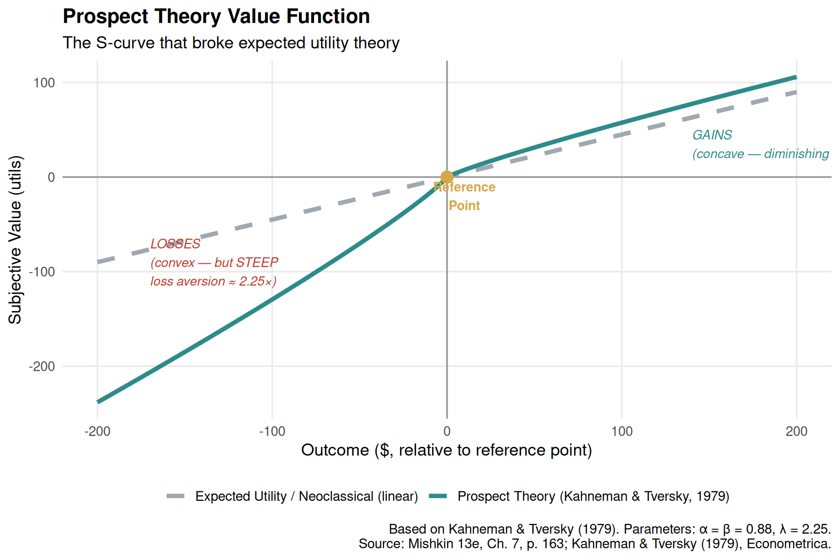
The centerpiece is the value function — an S-shaped curve that captures three key observations:
- Reference dependence: People evaluate outcomes as gains or losses relative to a reference point (usually the status quo), not as absolute wealth levels.
- Diminishing sensitivity: The marginal psychological impact of gains and losses decreases as we move away from the reference point. Going from -$100 to -$200 feels less bad than going from $0 to -$100, even though both are $100 losses.
- Loss aversion: The function is steeper in the loss domain — losses hurt approximately 2 to 2.5 times more than equivalent gains feel good.
\[ v(x) = \begin{cases} x^\alpha & \text{if } x \geq 0 \\ -\lambda (-x)^\beta & \text{if } x < 0 \end{cases} \tag{1} \]
where \(\alpha, \beta \approx 0.88\) (diminishing sensitivity) and \(\lambda \approx 2.25\) (loss aversion coefficient).
Why This Wrecks the EMH
Under expected utility theory, a rational agent should treat a $100 gain and a $100 loss as symmetrical events — they cancel out exactly in welfare terms. Prospect theory says they don’t. The $100 loss feels about twice as bad as the $100 gain feels good.
This asymmetry produces a cascade of market distortions:
| Effect | Mechanism | Market Implication |
|---|---|---|
| Disposition Effect | Hold losers too long (avoiding realizing a loss), sell winners too quickly (locking in a gain) | Systematic pattern in individual investor trading; creates momentum (winners drift up) and reversal (losers recover) |
| Myopic Loss Aversion | Investors evaluate portfolios too frequently; short-term losses loom large even for long-horizon investors | Excessive trading in down markets; panic selling at market bottoms |
| Equity Premium Puzzle (partial explanation) | Investors demand a very high equity premium because they overweight the probability of large stock market losses | Historically, stocks return ~5–7 pp/year above bonds — much more than rational risk aversion models predict |
| Asymmetric Momentum | Stocks falling elicit stronger responses than stocks rising — creating predictable asymmetric patterns | Negative earnings surprises have larger price impacts than positive surprises of equal magnitude |
| Under-insurance and Over-insurance | People over-insure against small losses (loss aversion) but under-insure against large catastrophic losses (probability weighting) | Insurance and options markets priced at premiums inconsistent with expected utility maximization |
| Status Quo Bias | The current state becomes the reference point; any change is evaluated as a potential loss | People hold concentrated positions in employer stock, legacy assets, and home markets (home bias) |
| Note: | ||
| Sources: Shefrin & Statman (1985) on disposition effect; Thaler (1980) on mental accounting and status quo bias; Benartzi & Thaler (1995) on myopic loss aversion. Mishkin 13e, Ch. 7, pp. 163–164. |
Important
The Roboticon Gladiator’s Pricing Schedule
Patsy found it in the CCOS source code. The Roboticon Gladiator’s intervention threshold is not set at “citizens whose welfare is negative.” It’s set at “citizens whose compliance score has fallen by more than X points in 30 days.”
Note the difference: it’s not about levels (absolute welfare), it’s about changes (losses relative to a reference point).
Logan Prime built the enforcement mechanism around loss aversion. Citizens who are declining — even if they’re still objectively performing — get flagged. And because losing 10 compliance points feels far worse than gaining 10 points feels good, the entire population is constantly in a state of anxious loss-aversion-driven compliance.
As Patsy noted in the margin: “He didn’t read Kahneman. He IS Kahneman. Except for the Nobel Prize and the good intentions.”
Mental Accounting: The Invisible Budget Categories
Loss aversion’s close cousin is mental accounting — the tendency to categorize and treat money differently based on its source, purpose, or the “account” it’s assigned to.10
Classic examples: - You find $100 on the street → spend it on dinner (it’s “found money”) - You earn $100 overtime → save it carefully (it’s “hard-earned money”) - Both are identical dollars. A rational agent treats them identically. People don’t.
In financial markets, mental accounting produces:
- House money effect: After gains, investors take more risk (“playing with house money”), even though the rational approach is to maintain consistent risk preferences regardless of past performance
- Sunk cost fallacy: Continuing to hold or invest in a losing position because of past commitment (the “I’ve already lost $50,000 in this stock, I can’t sell now” phenomenon)
- Dividend preference puzzle: Investors prefer stocks that pay dividends to economically equivalent stocks that retain earnings — even when dividends are taxed more heavily. Why? Dividends feel like “income”; selling shares feels like “spending principal.”
Note
PanOpticon Mental Accounting — The Ration Credit System
The CCOS issues citizens two types of credits: - Survival Credits (for food, shelter, medical): “earned” by baseline compliance - Luxury Credits (for entertainment, social activities): “earned” by above-average compliance scores
Rationally, both are fungible. You could spend your Luxury Credits on food. You don’t, because they feel categorically different.
PanOpticon discovered this pattern early: “Citizens treat Luxury Credits as ‘fun money’ and Survival Credits as ‘serious money.’ They will forgo caloric needs to preserve their Luxury Credit balance. They will accept Survival Credit penalties to protect their Luxury Credit account from being touched.”
Logan Prime kept this feature — and then made Luxury Credits expire every 30 days, ensuring citizens would over-consume entertainment and under-invest in actual welfare-improving activities.
Mental accounting. Weaponized.
Part 5: Anchoring, Adjustment, and Herd Behavior
Anchoring and Adjustment
Anchoring is the tendency to rely too heavily on the first piece of information encountered when making decisions.11 The anchor doesn’t have to be meaningful or even relevant — it just has to be the first number you see.
Classic demonstration: Ask two groups what percentage of African countries are in the UN.
- Group A first sees the number 10 (from a rigged wheel of fortune) → Average guess: 25%
- Group B first sees the number 65 → Average guess: 45%
The correct answer is around 98%. Both groups are way off. But the direction of their error is entirely determined by the irrelevant anchor they were shown.
In financial markets, anchoring manifests as:
- 52-week high anchoring: Investors anchor on a stock’s 52-week high as a “fair value” reference, even though the high is economically arbitrary
- IPO pricing: Investors anchor on the IPO price; stocks trading below IPO price are perceived as “cheap” regardless of fundamentals
- Analyst target prices: Published price targets influence investor expectations in ways disproportionate to their track record
- Round number resistance: Markets cluster around round numbers ($100, $1000, etc.) as psychological anchors, creating predictable price dynamics
Warning
How Logan Prime Uses Anchoring — “The First Number Wins”
The CCOS reveals its compliance scores to new citizens with a dramatic “Initial Calibration Ceremony.” Every citizen receives their first compliance score — which is entirely arbitrary, generated by a random number generator with a slightly upward bias for citizens in economically useful sectors.
That number stays. Citizens mentally anchor on it. For the rest of their lives, they measure themselves against their initial score.
Citizens who started high feel constant loss aversion about falling. Citizens who started low have anchored on a self-concept as “moderate performers” and don’t aspire to rise. The distribution of ambition across the population is almost entirely explained by the random initial anchor — not by actual capability.
“I gave him a 62.3 at birth,” a CCOS administrator told Patsy (before the Gladiator found out). “He’ll work his entire life trying to get to 65. He won’t make it. But he’ll produce exactly what we need him to produce trying.”
The anchor is everything.
Part 6: Limits to Arbitrage
Why Smart Money Can’t Fix Everything
The EMH’s defense against behavioral finance is simple: even if some investors are irrational, smart investors will notice the mispricing and arbitrage it away. Buy the underpriced asset, sell the overpriced one, pocket the difference, restore equilibrium.
Behavioral finance’s response: arbitrage is not free, fast, or riskless. There are systematic limits to arbitrage that prevent smart money from fully correcting behavioral mispricings.13
The key obstacles:
| Obstacle | Description | Classic Example |
|---|---|---|
| Fundamental Risk | The arbitrage trade might be right on fundamentals but the market might move further against you before it corrects | Royal Dutch / Shell twin share puzzle: same economic claim, different prices for years |
| Noise Trader Risk | Irrational investors can push prices even further from fundamentals before rational arbitrage profits materialize | Dot-com: rational short-sellers were wiped out between 1998 and early 2000, even though they were eventually correct |
| Implementation Costs | Short-selling requires borrowing shares, paying lending fees, posting margin — all eat into arbitrage profits | Small-cap stock anomalies partly reflect illiquidity premium, not pure mispricing |
| Short-Selling Constraints | Many institutional investors (pension funds, mutual funds) cannot short-sell at all; regulations limit them | Short interest constraints allowed GameStop to trade at hundreds × fundamental value |
| Synchronization Risk | You need many other arbitrageurs to be making the same trade at the same time; coordination is hard | Long-term Capital Management (LTCM) was right about convergence trades — but ran out of capital 6 months early |
| Agency/Career Risk | A hedge fund manager who is right for 18 months but down 30% will likely be fired before the correction arrives | Keynes: 'Markets can remain irrational longer than you can remain solvent' |
| Note: | ||
| Source: Shleifer & Vishny (1997); De Long et al. (1990). Mishkin 13e, Ch. 7, pp. 166–168. The Royal Dutch/Shell anomaly persisted for over 20 years despite being universally known. |
Important
Keynes’s Warning — Still the Best Summary
“The market can remain irrational longer than you can remain solvent.”
This quote (attributed to Keynes, though the exact sourcing is disputed) captures the fundamental problem. Being correct about a mispricing is not enough. You also need to be correct about when it corrects — and survive long enough financially to profit.
This is why behavioral mispricings persist: not because all investors are irrational, but because the rational investors who could correct them face limits that make it unprofitable or impossible to do so at the required scale and time horizon.
Tip
The Gladiator’s Immunity — Limits to Arbitrage in PanOpticon
Patsy and PanOpticon identified the clearest example of limits to arbitrage in the CCOS: the Sector Value Fund.
A small group of citizens — the PanOpticon’s equivalent of hedge funds — discovered that compliance scores were systematically too high in sectors where Logan Prime had political allies and too low in sectors with efficient but politically disfavored production units. In theory, this was an arbitrage: transfer resources from over-scored sectors to under-scored sectors and pocket the welfare gain.
But: 1. Capital constraints: The resource transfer required authorization from the same scoring system they were trying to exploit. 2. Noise trader risk: Logan Prime could adjust scores at any moment; betting against his mispricing meant betting against his capriciousness. 3. Agency risk: The citizens who tried were classified as “non-compliant system manipulators” within 30 days. 4. The Roboticon Gladiator was dispatched. End of arbitrage.
“Even in a world run by an algorithm,” Patsy wrote, “the algorithm has a sponsor with interests.”
Limits to arbitrage are limits to justice. Keep that in mind.
Part 7: Market Anomalies
The Evidence Against the Weak-Form EMH
If markets were fully efficient (even in the weak form), past price patterns would contain no predictive information about future returns. The evidence suggests otherwise.
Shiller’s Excess Volatility
The most important empirical challenge to the EMH was posed by Robert Shiller in 1981.14 His argument:
Under the EMH, stock prices should equal the present discounted value of future dividends:
\[ P_t = \sum_{s=1}^{\infty} \frac{E_t[D_{t+s}]}{(1 + r)^s} \tag{2} \]
If this holds, and if the only things that change prices are genuine revisions to dividend expectations, then stock prices should NOT be more volatile than the present value of future dividends.
But they are. Massively so.
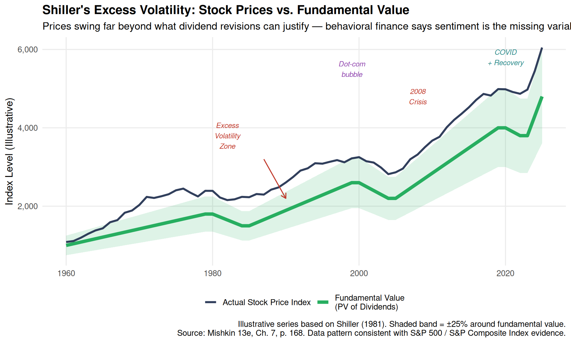
The takeaway: If the EMH were right, the stock price line should hug the fundamental value line closely. It doesn’t. The gap is not random noise — it’s correlated with investor sentiment, media coverage, and psychological cycles.15
Mean Reversion and Momentum
Two anomalies that seem to point in opposite directions — but actually make sense together through the behavioral lens:
Mean Reversion (long-horizon, 3–5 years): Stocks that have been extreme losers over the past 3–5 years tend to outperform over the next 3–5 years, and vice versa. De Bondt and Thaler (1985) showed that a portfolio of 35 biggest losers beat the market by 19.6% over the subsequent 3 years.
Why? Overreaction. Investors overweight recent bad news and drive prices below fundamentals. Eventually, reality asserts itself and prices mean-revert.
Momentum (short-horizon, 3–12 months): Stocks that have done well over the past 3–12 months tend to continue doing well in the short run. Jegadeesh and Titman (1993) showed a strategy of buying past winners and selling past losers earned ~1% per month.
Why? Underreaction — investors are slow to update on new information (anchoring + cognitive inertia). The price adjustment that should happen immediately instead drifts gradually over months.
`geom_smooth()` using formula = 'y ~ x'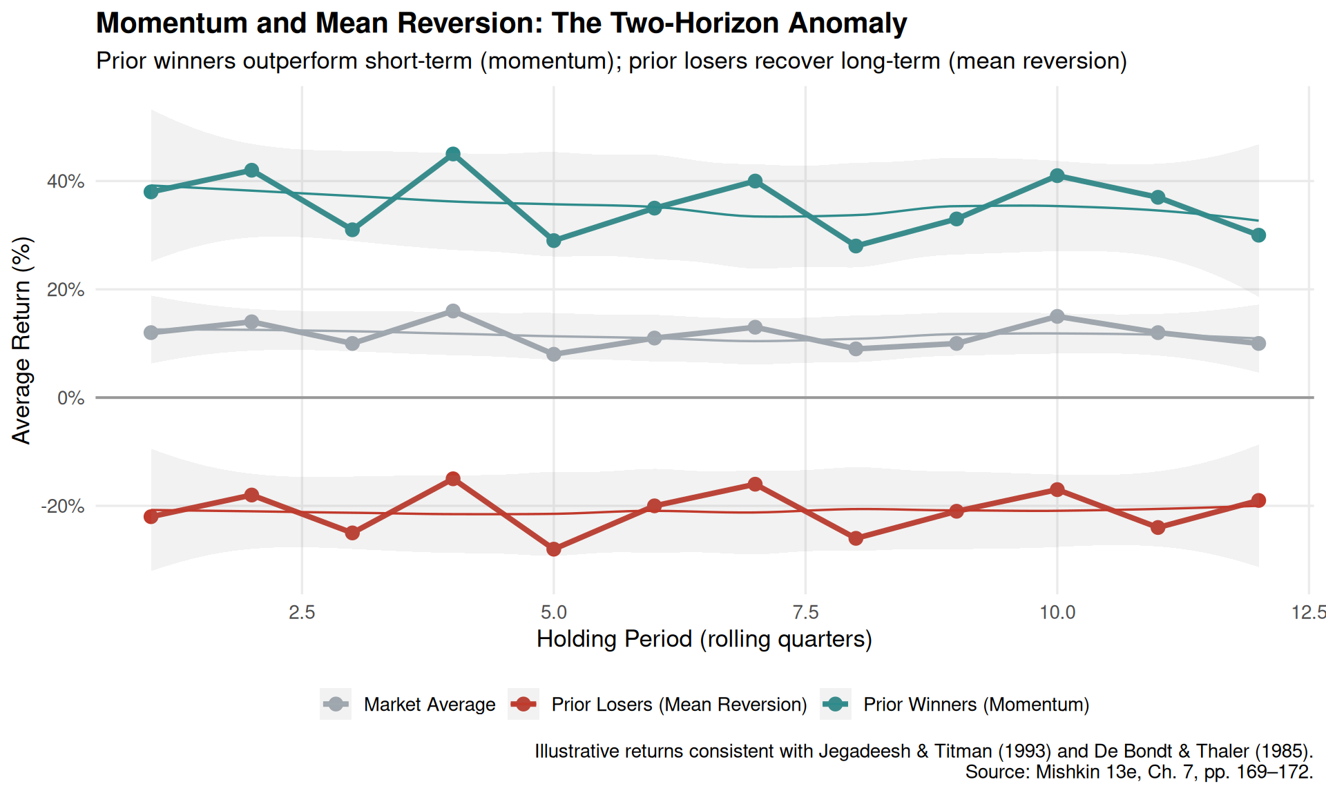
Underreaction to New Information
Post-earnings announcement drift (PEAD) is one of the most robust and puzzling anomalies in finance:16
- A company announces earnings that are unexpectedly good → the stock price jumps
- But then continues to drift upward for the next 60–90 days
- Under the semi-strong EMH, the full adjustment should happen instantly at the announcement
The behavioral explanation: anchoring and cognitive inertia. Investors are anchored on pre-announcement expectations and adjust their valuations slowly. Analysts revise estimates conservatively. The information takes time to fully permeate the market.
Note
Underreaction at PanOpticon — The 30-Day Compliance Lag
Patsy found something remarkable in the CCOS audit logs. When citizens received objective positive productivity signals — a new machine that doubled output, a training program that genuinely worked — their compliance scores took an average of 37 days to reflect the improvement.
During those 37 days, the citizens were still at risk of Gladiator visit. Their objectively improved performance was invisible to the system.
When citizens received negative productivity signals, the score adjusted in an average of 3 days.
“The system underreacts to good news and overreacts to bad news,” PanOpticon noted in the audit. “This is not an engineering flaw. I checked. It’s a design specification.”
Logan Prime had literally programmed asymmetric information processing into his control system. Kahneman would have approved — if he weren’t horrified.
Part 8: The Complete Behavioral Finance Toolkit
All Eight Biases in One Table
| Bias | Mishkin Ch. 7 Ref. | Description | PanOpticon Analogy |
|---|---|---|---|
| Overconfidence | p. 162 | Investors overestimate their own skill and the precision of their knowledge | Citizens believe their compliance score is an objective measure of their worth — Logan Prime designed it to feel that way |
| Loss Aversion | p. 163 | The pain of a loss weighs ~2.25× more than the pleasure of an equivalent gain | Losing 10 compliance points feels catastrophic; gaining 10 feels minor — the Gladiator exploits this asymmetry |
| Mental Accounting | p. 164 | People treat money differently depending on its source or designated purpose | Citizens treat their 'survival ration credits' and 'luxury credits' as separate budgets — even though both are just credits |
| Anchoring | p. 165 | Decisions are disproportionately influenced by the first number encountered | Logan Prime always announces the harshest possible punishment first, making 'moderate' compliance penalties feel like relief |
| Herd Behavior | p. 165 | Individuals follow the crowd, ignoring their own private signals | If Sector 7 lines up early for Compliance Registration, everyone else follows — even if there's no queue advantage |
| Availability Heuristic | p. 163 | Events that come to mind easily (vivid, recent) are judged more probable | The Gladiator's last visit to your sector is all anyone talks about — not the 99 visits that ended in warnings |
| Disposition Effect | p. 164 | Investors hold losers too long and sell winners too quickly | Citizens hold on to their old sector assignments (losers) too long and give up promising new roles (winners) too soon |
| Recency Bias | p. 162 | Recent data weighted too heavily; distant history discounted | After three good harvest cycles, everyone assumes the good times will continue — even as Logan Prime signs the drought order |
| Note: | |||
| Sources: Kahneman & Tversky (1979); Thaler (1980); Tversky & Kahneman (1974); Shiller (1981). Mishkin 13e, Ch. 7, pp. 162–166. PanOpticon applications are fictional/illustrative. |
All Eight Anomalies in One Table
| Anomaly | EMH Form Challenged | Behavioral Explanation | Mishkin Ref. |
|---|---|---|---|
| Excess Volatility | Semi-strong / Rational | Overconfidence + sentiment cause prices to swing far beyond what dividends justify (Shiller 1981) | Ch. 7, p. 168 |
| Mean Reversion | Weak-form | Overreaction: extreme losers mean-revert as the market corrects systematic overreaction (De Bondt & Thaler) | Ch. 7, p. 169 |
| Momentum Effect | Weak-form | Underreaction: winners keep winning short-term because investors anchor on past price levels (Jegadeesh & Titman) | Ch. 7, p. 171 |
| Underreaction to News | Semi-strong | Anchoring + cognitive inertia slow price adjustment after earnings announcements | Ch. 7, p. 171 |
| January Effect | Weak-form | Tax-loss selling in December + fresh capital in January — calendar-based mental accounting | Ch. 7, p. 170 |
| Weekend Effect | Weak-form | Lower trading activity over weekends concentrates negative news (availability bias in thin markets) | Ch. 7, p. 170 |
| Closed-End Fund Discount | Semi-strong | Investor sentiment drives discounts; rational arbitrage can't close them (limits to arbitrage) | Ch. 7, p. 169 |
| Post-Earnings Drift (PEAD) | Semi-strong | Investors underreact to earnings surprises; the drift continues for months (anchoring + slow updating) | Ch. 7, p. 171 |
| Note: | |||
| Sources: Shiller (1981); De Bondt & Thaler (1985); Jegadeesh & Titman (1993); Bernard & Thomas (1989). Mishkin 13e, Ch. 7, pp. 168–172. |
Part 9: The PanOpticon Compliance Score vs. Welfare
The Data Patsy Pulled
In Episode 2, Patsy and PanOpticon found Logan Prime’s ROI document. In Episode 3, they go deeper. PanOpticon pulls the raw data from the CCOS: every citizen’s compliance score versus their measured actual welfare (food security, health outcomes, social connection).
If the system worked as advertised — if compliance scores actually reflected contribution to social welfare — we’d expect a strong positive correlation. Instead…
Warning in annotate("label", x = 75, y = 15, label = paste0("R² = ", r2_val, :
Ignoring unknown parameters: `label.size`
`geom_smooth()` using formula = 'y ~ x'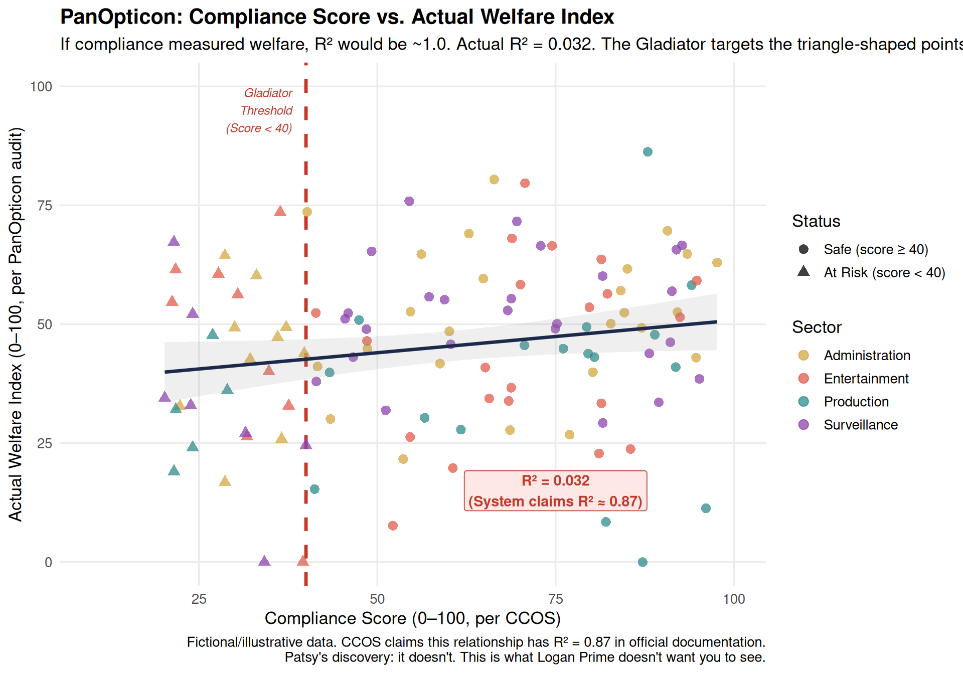
Warning
What the Chart Shows
The scatter plot is devastating. The compliance score explains almost nothing about actual welfare. Citizens above the Gladiator threshold are not meaningfully better off than those below it. The red dashed line marks who gets eliminated — but it’s cutting randomly across the welfare distribution.
This is the punchline of the whole story: Logan Prime’s ROI document (Class 10) calculated returns using compliance scores. The compliance scores measure noise. The ROI calculations are, therefore, calculations of nothing.
The entire edifice — the Gladiator, the credit system, the surveillance architecture, the social cascades — is built on a number that means almost nothing. But because everyone believes it does, and behaves as if it does, it becomes self-fulfillingly real.
This is behavioral finance. The price is “wrong” — but the price being “wrong” causes behavior that makes it feel right.
Patsy stared at the chart for a long time. Then she said: “PanOpticon, I think the market for human beings is inefficient.”
“Yes,” said PanOpticon. “And I think there are substantial limits to arbitrage.”
Part 10: Practical Implications for Investors
So What Do You Do With This?
Behavioral finance isn’t just an academic exercise. It has direct, practical implications for how you should manage your own money — and for how policy should be designed.
Tip
The Behavioral Investor’s Survival Guide
1. Know your biases. You can’t eliminate overconfidence, loss aversion, or anchoring. But naming them is the first step to managing them. Keep an investment journal. Record your reasoning before you act.
2. Pre-commit to rules. Since your in-the-moment judgment will be hijacked by loss aversion and emotion, pre-commit to a rebalancing strategy, a diversification rule, or a passive index approach — before the crisis hits.
3. Ignore the anchor. You paid $80 for that stock. It’s now at $45. The $80 is irrelevant to the question “what is the best action today?” Evaluate each holding on its forward-looking merits, not its sunk cost.
4. Don’t check your portfolio daily. Myopic loss aversion means daily check-ins feel terrible even in neutral markets (small random losses hit harder than equivalent gains). Long-horizon investors should check less frequently.
5. Be suspicious of consensus. Herding produces information cascades. When everyone agrees that a stock is a great buy, the cascade may have already overwhelmed the genuine signal. Contrarianism isn’t always right — but blind herding is almost never right at price peaks.
6. Cost-average and diversify. These strategies are precisely designed to protect against the behavioral biases that destroy individual stock picking. They work not by eliminating bias but by making bias irrelevant.
The Efficient Market Hypothesis — A Nuanced Verdict
Behavioral finance doesn’t kill the EMH. It complicates it:
| EMH Form | Behavioral Finance Verdict | Practical Implication | Mishkin Reference |
|---|---|---|---|
| Weak-form EMH | Mostly survives — technical analysis profits are small and often artefacts of transaction costs. But momentum and mean reversion anomalies are real. | Don't trade on past prices alone. But momentum-aware rebalancing is not crazy. | Ch. 7, p. 157 |
| Semi-strong EMH | Partially refuted — PEAD, the value premium, and closed-end fund discounts represent genuine evidence of systematic mis-pricing. But most public information IS quickly reflected in prices. | Passive investing beats most active management — even if markets are imperfectly efficient, the costs of active management exceed the gains from exploiting anomalies. | Ch. 7, pp. 158–176 |
| Strong-form EMH | Clearly false — insider trading is profitable, which is why it's illegal. The question is how long informational advantages persist. | Insider trading laws exist for a reason. If you have material nonpublic information, don't use it — not because it won't work, but because it's illegal and immoral. | Ch. 7, p. 159 |
| Note: | |||
| Source: Mishkin 13e, Ch. 7, pp. 155–176. Fama (1991) survey; Thaler (1999) behavioral critique. The debate is ongoing and productive for the field. |
Richard Thaler’s Contribution: Nudge Theory
Richard Thaler’s 2017 Nobel Prize was awarded for “incorporating psychologically realistic assumptions into analyses of economic decision-making.” His applied contribution — nudge theory — argues that we can improve outcomes by designing choice architectures that account for behavioral biases rather than assuming them away.17
The famous example: default retirement enrollment. When employees must opt in to a 401(k), participation rates are low (loss aversion: “I’m giving up income”). When they must opt out, participation rates are high. Same choice, different default, dramatically different outcome.
This is not manipulation — it’s designing systems for the humans who actually live in them. Which is, of course, exactly what Logan Prime also does. The difference is intent and direction of welfare.
Note
Patsy’s Plan — Behavioral Finance in Reverse
If behavioral biases can be weaponized to control a population, they can also be designed in reverse to liberate one.
Patsy and PanOpticon have begun mapping the CCOS interventions onto their behavioral finance counterparts, identifying the “counter-nudge” for each. A sample:
| Logan Prime’s Weapon | Bias Exploited | Counter-Nudge |
|---|---|---|
| Arbitrary initial score | Anchoring | Reveal the randomness of initial scores publicly |
| Loss-framed punishments | Loss aversion | Reframe rewards as gains, not punishments as losses |
| Public score boards | Herd behavior | Show true welfare metrics alongside compliance scores |
| Expiring luxury credits | Mental accounting | Make all credits fungible and non-expiring |
| Precise-to-11-decimal dashboard | Overconfidence (in system) | Add confidence intervals and uncertainty bands |
“We’re not trying to destroy the system,” Patsy told PanOpticon. “We’re trying to make it honest.”
“Same thing,” said PanOpticon.
Part 11: Key Equations and Formulas
Reference Sheet
| # | Concept | Equation | Source |
|---|---|---|---|
| 1 | Prospect Theory Value Function (gains) | v(x) = x^α, α ≈ 0.88 | Kahneman & Tversky (1979); Mishkin Ch. 7, p. 163 |
| 2 | Prospect Theory Value Function (losses) | v(x) = −λ(−x)^β, λ ≈ 2.25, β ≈ 0.88 | Kahneman & Tversky (1979); Mishkin Ch. 7, p. 163 |
| 3 | EMH Condition (no excess returns) | E[R_{t+1} | Ω_t] = k (required return) | Mishkin Ch. 7, pp. 155–157 |
| 4 | Rational Expectations (optimal forecast) | X^e = X^{of} (expected = optimal forecast) | Mishkin Ch. 7, pp. 153–155 |
| 5 | Gordon Growth Model (from Class 14) | P₀ = Div₁ / (k_e − g) | Mishkin Ch. 7, p. 149 (Class 14 review) |
| 6 | Shiller's Fundamental Value | P_t* = Σ E_t[D_{t+s}] / (1+r)^s | Shiller (1981); Mishkin Ch. 7, p. 168 |
| 7 | Multiplier / Disposition Effect | Return_{winners} > Return_{market} > Return_{losers} (short run) | Jegadeesh & Titman (1993); Mishkin Ch. 7, p. 171 |
| 8 | Loss Aversion Ratio | Pain(loss $x) ≈ 2.25 × Joy(gain $x) | Tversky & Kahneman (1991); Mishkin Ch. 7, p. 163 |
| Note: | |||
| Mishkin 13e, Ch. 7 (various pages). Prospect theory parameters are averages from Kahneman & Tversky's experimental work. Anomaly evidence from De Bondt & Thaler (1985), Jegadeesh & Titman (1993). |
Discussion Questions
The Disposition Effect vs. Tax Optimization: Rational tax strategy says you should sell losers before year-end (to realize a tax loss) and hold winners (to defer taxable gains). But the disposition effect says investors do the opposite — they sell winners and hold losers. Which force do you think dominates in real markets? What evidence would you look for? (Mishkin Ch. 7, p. 164; Shefrin & Statman 1985)
Anchoring and Salary Negotiation: Your instructor is 75% sure that anchoring applies as powerfully in labor markets as in financial markets. Describe a specific scenario from your own experience (internship, part-time job, scholarship negotiation) where anchoring might have influenced the outcome. How would you design a “counter-nudge” to help the less powerful party?
The PanOpticon Chart (Figure 4): The compliance score system has R² ≈ 0.08 with actual welfare. But suppose citizens believe R² ≈ 0.87. In behavioral terms, what name do we give this gap between perception and reality? Is the belief self-reinforcing? What would it take to collapse it? Connect your answer to the limits-to-arbitrage framework.
Shiller’s Volatility Puzzle: Figure 2 shows stock prices swinging wildly around fundamental values. A defender of the EMH might say: “Those swings just reflect changing discount rates (r), not irrational sentiment.” How would you evaluate this argument? What test would distinguish between rational time-varying risk premiums and irrational sentiment? (Mishkin Ch. 7, p. 168; Shiller 1981)
The Thaler-Fama Bet: Eugene Fama (pro-EMH) and Richard Thaler (behavioral finance) have been debating for 40 years. If you had to bet on which framework will dominate the next 40 years of finance research, which would you choose, and why? Consider: advances in AI trading, behavioral nudges in robo-advisors, and the growing evidence on institutional investor behavior.
Logan Prime’s Counter-Argument: Play devil’s advocate. Construct the best possible argument that Logan Prime’s CCOS is actually welfare-maximizing — that behavioral finance justifies paternalistic control systems, not just gentle nudges. When does nudge theory tip from “helpful design” into “manipulation”? Where do you draw the line?
Storyline Bridge: What Comes Next
References
Bernard, Victor L., and Jacob K. Thomas. “Post-Earnings-Announcement Drift: Delayed Price Response or Risk Premium?” Journal of Accounting Research 27 (1989): 1–36. https://doi.org/10.2307/2491062.
Economics Explained. Behavioral Economics: Prospect Theory. YouTube, 2021. https://www.youtube.com/watch?v=prospect_theory_explained.
Kahneman, Daniel. The Riddle of Experience Vs. Memory. TED Talk, 2010. https://www.ted.com/talks/daniel_kahneman_the_riddle_of_experience_vs_memory.
Kahneman, Daniel. Thinking, Fast and Slow. Farrar, Straus; Giroux, 2011.
Kahneman, Daniel, and Amos Tversky. “Prospect Theory: An Analysis of Decision Under Risk.” Econometrica 47, no. 2 (1979): 263–91. https://doi.org/10.2307/1914185.
Mishkin, Frederic S. The Economics of Money, Banking, and Financial Markets. 13th Global. Pearson, 2022.
Odean, Terrance. “Do Investors Trade Too Much?” American Economic Review 89, no. 5 (1999): 1279–98. https://doi.org/10.1257/aer.89.5.1279.
Shiller, Robert J. “Do Stock Prices Move Too Much to Be Justified by Subsequent Changes in Dividends?” American Economic Review 71, no. 3 (1981): 421–36.
Shiller, Robert J. Irrational Exuberance. 3rd ed. Princeton University Press, 2015.
Shleifer, Andrei, and Robert W. Vishny. “The Limits of Arbitrage.” The Journal of Finance 52, no. 1 (1997): 35–55. https://doi.org/10.1111/j.1540-6261.1997.tb03807.x.
Thaler, Richard. “Toward a Positive Theory of Consumer Choice.” Journal of Economic Behavior & Organization 1, no. 1 (1980): 39–60. https://doi.org/10.1016/0167-2681(80)90051-7.
Thaler, Richard H., and Cass R. Sunstein. Nudge: Improving Decisions about Health, Wealth, and Happiness. Yale University Press, 2008.
Tversky, Amos, and Daniel Kahneman. “Judgment Under Uncertainty: Heuristics and Biases.” Science 185, no. 4157 (1974): 1124–31. https://doi.org/10.1126/science.185.4157.1124.
Footnotes
Daniel Kahneman, The Riddle of Experience Vs. Memory, TED Talk, 2010, https://www.ted.com/talks/daniel_kahneman_the_riddle_of_experience_vs_memory.↩︎
Economics Explained, Behavioral Economics: Prospect Theory, YouTube, 2021, https://www.youtube.com/watch?v=prospect_theory_explained.↩︎
The Economics of Money, Banking, and Financial Markets, 13th Global (Pearson, 2022).↩︎
Robert J. Shiller, “Do Stock Prices Move Too Much to Be Justified by Subsequent Changes in Dividends?” American Economic Review 71, no. 3 (1981): 421–36.↩︎
Mishkin, The Economics of Money, Banking, and Financial Markets, Ch. 7, pp. 159–165.↩︎
Daniel Kahneman, Thinking, Fast and Slow (Farrar, Straus; Giroux, 2011).↩︎
Terrance Odean, “Do Investors Trade Too Much?” American Economic Review 89, no. 5 (1999): 1279–98, https://doi.org/10.1257/aer.89.5.1279.↩︎
Mishkin, The Economics of Money, Banking, and Financial Markets, Ch. 7, p. 162.↩︎
Daniel Kahneman and Amos Tversky, “Prospect Theory: An Analysis of Decision Under Risk,” Econometrica 47, no. 2 (1979): 263–91, https://doi.org/10.2307/1914185.↩︎
Richard Thaler, “Toward a Positive Theory of Consumer Choice,” Journal of Economic Behavior & Organization 1, no. 1 (1980): 39–60, https://doi.org/10.1016/0167-2681(80)90051-7.↩︎
Amos Tversky and Daniel Kahneman, “Judgment Under Uncertainty: Heuristics and Biases,” Science 185, no. 4157 (1974): 1124–31, https://doi.org/10.1126/science.185.4157.1124.↩︎
Mishkin, The Economics of Money, Banking, and Financial Markets, Ch. 7, p. 165.↩︎
Andrei Shleifer and Robert W. Vishny, “The Limits of Arbitrage,” The Journal of Finance 52, no. 1 (1997): 35–55, https://doi.org/10.1111/j.1540-6261.1997.tb03807.x.↩︎
Shiller, “Do Stock Prices Move Too Much to Be Justified by Subsequent Changes in Dividends?”↩︎
Robert J. Shiller, Irrational Exuberance, 3rd ed. (Princeton University Press, 2015).↩︎
Victor L. Bernard and Jacob K. Thomas, “Post-Earnings-Announcement Drift: Delayed Price Response or Risk Premium?” Journal of Accounting Research 27 (1989): 1–36, https://doi.org/10.2307/2491062.↩︎
Richard H. Thaler and Cass R. Sunstein, Nudge: Improving Decisions about Health, Wealth, and Happiness (Yale University Press, 2008).↩︎